2 Introducción a R
R es un elenguaje de programación. Además es un entorno integrado para el manejo de datos, el cálculo, la generación de gráficos y análisis estadísticos. Las principales ventajas del uso de R son:
- Es software libre.
- Su facilidad para el manejo y almacenamiento de datos.
- Es un conjunto de operadores para el cálculo de vectores y matrices.
- Es una colección extensa e integrada de herramientas intermedias para el análisis estadístico de datos.
- Posee un multitud de facilidades gráficas de altísima calidad
- Es un lenguaje de programación (muy) poderoso con muchas librerías , bibliotecas más porpiamente dicho, especializadas disponibles.
- La mejor herramienta para trabajar con datos genómicos, proteomicos, redes, metabolómica, entre varias más.
- Casi todos podemos aprender por nuestra cuenta a usar excel (pero hay que pagar por la licencia…), sin embargo es más díficil aprender por nuestra cuenta R; y si lo hacemos nos da una ventaja sobre el resto.
2.1 Paquetes o bibliotecas
Las funciones especializadas de R se guardan en bibliotecas (packages) que deben ser invocados ANTES de llamar a una función de la biblioteca
Una manera de instalar bibliotecas es mediante el repositorio por defecto de R que es CRAN.
Navega por CRAN y encuentra algunos paquetes que podrían interesarte. Hay miles y cada día aumentan.
Para saber qué paquetes se tienen instalados en tu máquina teclea la función library()
library()Para cargar un paquete en particular deben teclear, siempre y cuando ya esté instalado
Por ejemplo
##
## Attaching package: 'gplots'
## The following object is masked from 'package:stats':
##
## lowessPara visualizar los paquetes ya cargados tecleamos
search()## [1] ".GlobalEnv" "package:gplots" "package:stats"
## [4] "package:graphics" "package:grDevices" "package:utils"
## [7] "package:datasets" "package:methods" "Autoloads"
## [10] "package:base"Para visualizar las funciones dentro de un paquete en particular se utiliza
ls(2)## [1] "angleAxis" "balloonplot" "bandplot" "barplot2"
## [5] "bluered" "boxplot2" "ci2d" "col2hex"
## [9] "colorpanel" "greenred" "heatmap.2" "hist2d"
## [13] "lmplot2" "lowess" "ooplot" "overplot"
## [17] "panel.overplot" "plot.venn" "plotCI" "plotLowess"
## [21] "plotmeans" "qqnorm.aov" "redblue" "redgreen"
## [25] "reorder.factor" "residplot" "rich.colors" "sinkplot"
## [29] "smartlegend" "space" "textplot" "venn"
## [33] "wapply"
demo(graphics)##
##
## demo(graphics)
## ---- ~~~~~~~~
##
## > # Copyright (C) 1997-2009 The R Core Team
## >
## > require(datasets)
##
## > require(grDevices); require(graphics)
##
## > ## Here is some code which illustrates some of the differences between
## > ## R and S graphics capabilities. Note that colors are generally specified
## > ## by a character string name (taken from the X11 rgb.txt file) and that line
## > ## textures are given similarly. The parameter "bg" sets the background
## > ## parameter for the plot and there is also an "fg" parameter which sets
## > ## the foreground color.
## >
## >
## > x <- stats::rnorm(50)
##
## > opar <- par(bg = "white")
##
## > plot(x, ann = FALSE, type = "n")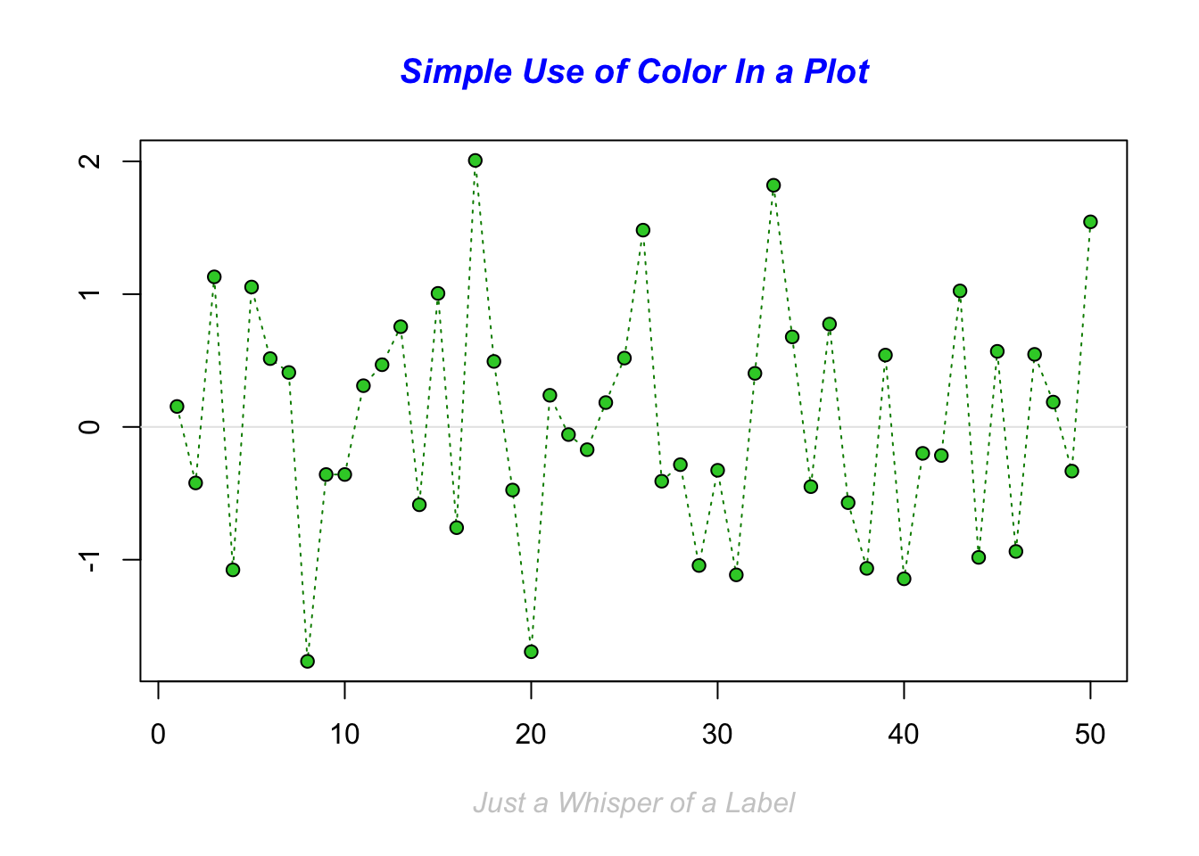
##
## > abline(h = 0, col = gray(.90))
##
## > lines(x, col = "green4", lty = "dotted")
##
## > points(x, bg = "limegreen", pch = 21)
##
## > title(main = "Simple Use of Color In a Plot",
## +       xlab = "Just a Whisper of a Label",
## +       col.main = "blue", col.lab = gray(.8),
## +       cex.main = 1.2, cex.lab = 1.0, font.main = 4, font.lab = 3)
##
## > ## A little color wheel.    This code just plots equally spaced hues in
## > ## a pie chart.    If you have a cheap SVGA monitor (like me) you will
## > ## probably find that numerically equispaced does not mean visually
## > ## equispaced.  On my display at home, these colors tend to cluster at
## > ## the RGB primaries.  On the other hand on the SGI Indy at work the
## > ## effect is near perfect.
## >
## > par(bg = "gray")
##
## > pie(rep(1,24), col = rainbow(24), radius = 0.9)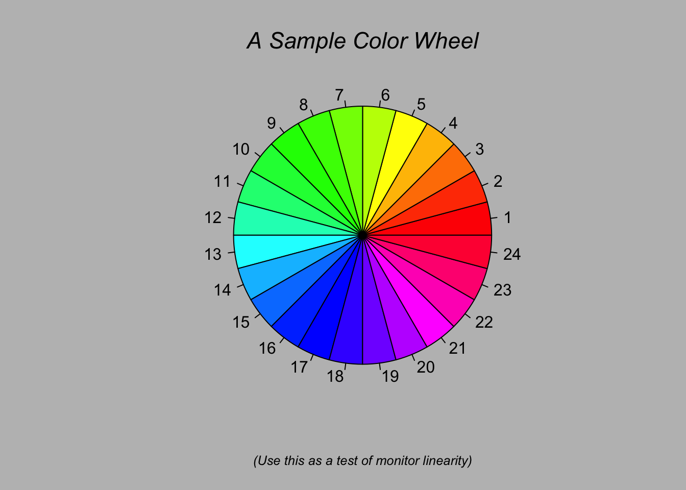
##
## > title(main = "A Sample Color Wheel", cex.main = 1.4, font.main = 3)
##
## > title(xlab = "(Use this as a test of monitor linearity)",
## +       cex.lab = 0.8, font.lab = 3)
##
## > ## We have already confessed to having these.  This is just showing off X11
## > ## color names (and the example (from the postscript manual) is pretty "cute".
## >
## > pie.sales <- c(0.12, 0.3, 0.26, 0.16, 0.04, 0.12)
##
## > names(pie.sales) <- c("Blueberry", "Cherry",
## +              "Apple", "Boston Cream", "Other", "Vanilla Cream")
##
## > pie(pie.sales,
## +     col = c("purple","violetred1","green3","cornsilk","cyan","white"))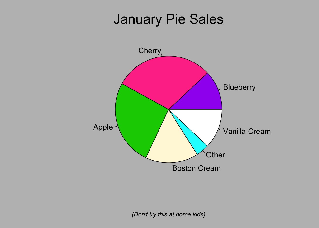
##
## > title(main = "January Pie Sales", cex.main = 1.8, font.main = 1)
##
## > title(xlab = "(Don't try this at home kids)", cex.lab = 0.8, font.lab = 3)
##
## > ## Boxplots:  I couldn't resist the capability for filling the "box".
## > ## The use of color seems like a useful addition, it focuses attention
## > ## on the central bulk of the data.
## >
## > par(bg="cornsilk")
##
## > n <- 10
##
## > g <- gl(n, 100, n*100)
##
## > x <- rnorm(n*100) + sqrt(as.numeric(g))
##
## > boxplot(split(x,g), col="lavender", notch=TRUE)
##
## > title(main="Notched Boxplots", xlab="Group", font.main=4, font.lab=1)
##
## > ## An example showing how to fill between curves.
## >
## > par(bg="white")
##
## > n <- 100
##
## > x <- c(0,cumsum(rnorm(n)))
##
## > y <- c(0,cumsum(rnorm(n)))
##
## > xx <- c(0:n, n:0)
##
## > yy <- c(x, rev(y))
##
## > plot(xx, yy, type="n", xlab="Time", ylab="Distance")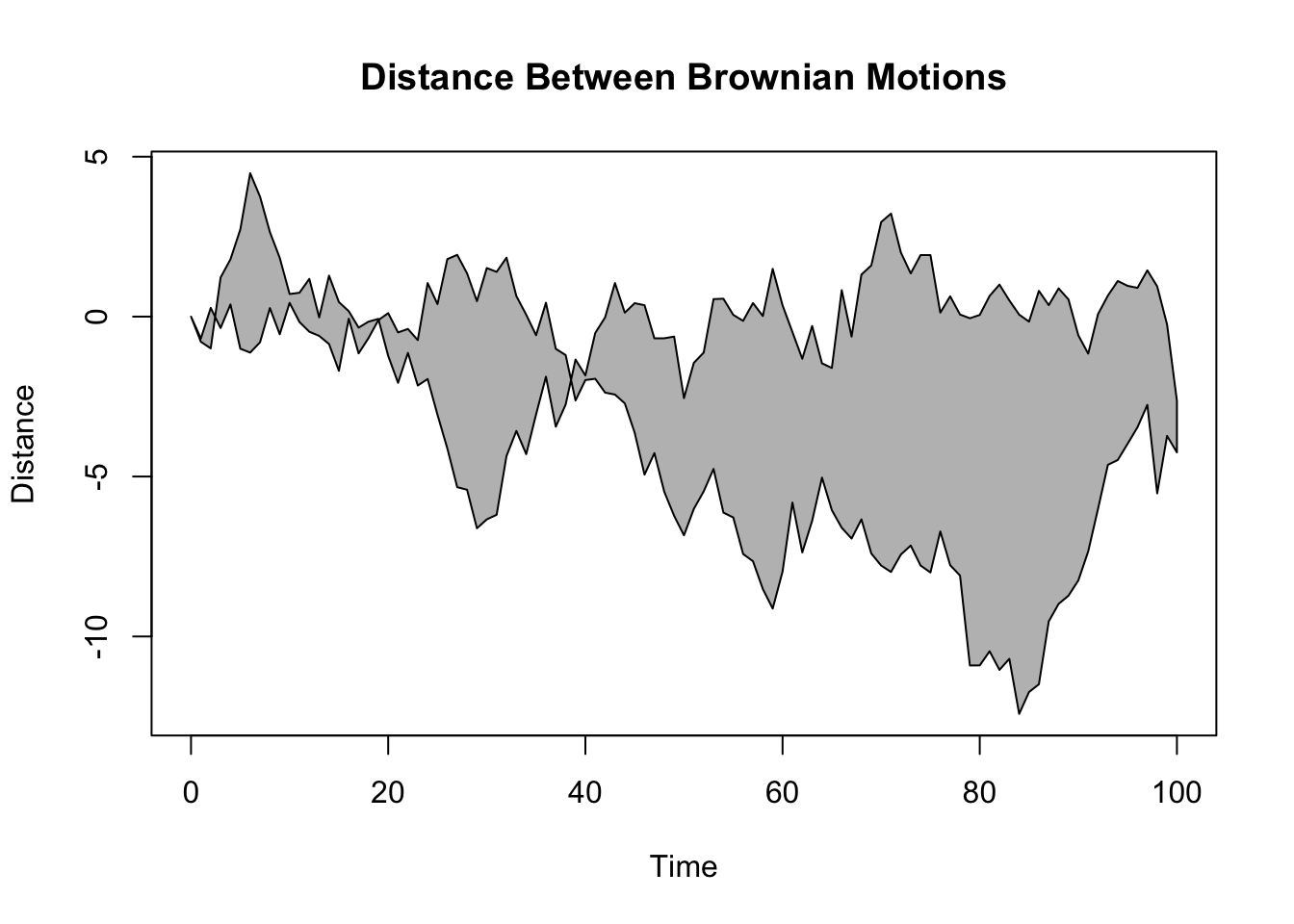
##
## > polygon(xx, yy, col="gray")
##
## > title("Distance Between Brownian Motions")
##
## > ## Colored plot margins, axis labels and titles.    You do need to be
## > ## careful with these kinds of effects.    It's easy to go completely
## > ## over the top and you can end up with your lunch all over the keyboard.
## > ## On the other hand, my market research clients love it.
## >
## > x <- c(0.00, 0.40, 0.86, 0.85, 0.69, 0.48, 0.54, 1.09, 1.11, 1.73, 2.05, 2.02)
##
## > par(bg="lightgray")
##
## > plot(x, type="n", axes=FALSE, ann=FALSE)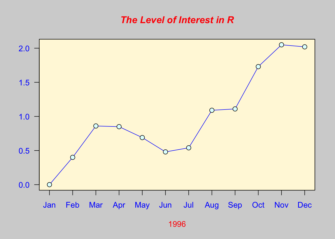
##
## > usr <- par("usr")
##
## > rect(usr[1], usr[3], usr[2], usr[4], col="cornsilk", border="black")
##
## > lines(x, col="blue")
##
## > points(x, pch=21, bg="lightcyan", cex=1.25)
##
## > axis(2, col.axis="blue", las=1)
##
## > axis(1, at=1:12, lab=month.abb, col.axis="blue")
##
## > box()
##
## > title(main= "The Level of Interest in R", font.main=4, col.main="red")
##
## > title(xlab= "1996", col.lab="red")
##
## > ## A filled histogram, showing how to change the font used for the
## > ## main title without changing the other annotation.
## >
## > par(bg="cornsilk")
##
## > x <- rnorm(1000)
##
## > hist(x, xlim=range(-4, 4, x), col="lavender", main="")
##
## > title(main="1000 Normal Random Variates", font.main=3)
##
## > ## A scatterplot matrix
## > ## The good old Iris data (yet again)
## >
## > pairs(iris[1:4], main="Edgar Anderson's Iris Data", font.main=4, pch=19)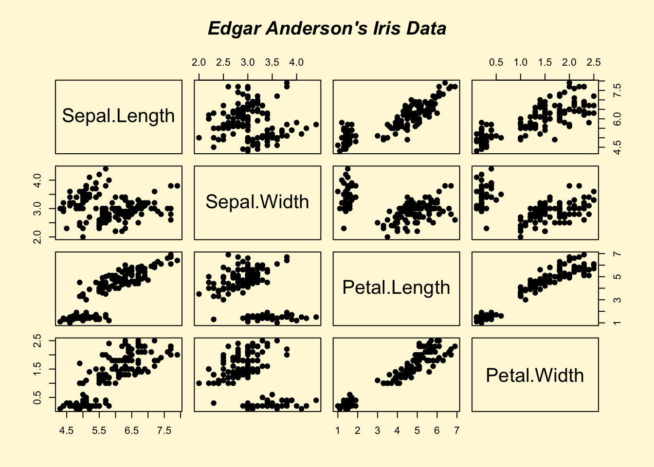
##
## > pairs(iris[1:4], main="Edgar Anderson's Iris Data", pch=21,
## +       bg = c("red", "green3", "blue")[unclass(iris$Species)])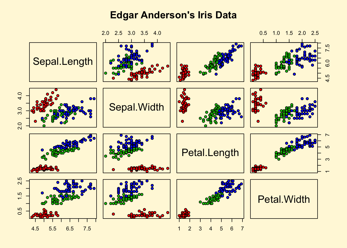
##
## > ## Contour plotting
## > ## This produces a topographic map of one of Auckland's many volcanic "peaks".
## >
## > x <- 10*1:nrow(volcano)
##
## > y <- 10*1:ncol(volcano)
##
## > lev <- pretty(range(volcano), 10)
##
## > par(bg = "lightcyan")
##
## > pin <- par("pin")
##
## > xdelta <- diff(range(x))
##
## > ydelta <- diff(range(y))
##
## > xscale <- pin[1]/xdelta
##
## > yscale <- pin[2]/ydelta
##
## > scale <- min(xscale, yscale)
##
## > xadd <- 0.5*(pin[1]/scale - xdelta)
##
## > yadd <- 0.5*(pin[2]/scale - ydelta)
##
## > plot(numeric(0), numeric(0),
## +      xlim = range(x)+c(-1,1)*xadd, ylim = range(y)+c(-1,1)*yadd,
## +      type = "n", ann = FALSE)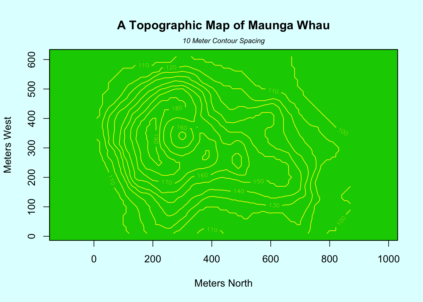
##
## > usr <- par("usr")
##
## > rect(usr[1], usr[3], usr[2], usr[4], col="green3")
##
## > contour(x, y, volcano, levels = lev, col="yellow", lty="solid", add=TRUE)
##
## > box()
##
## > title("A Topographic Map of Maunga Whau", font= 4)
##
## > title(xlab = "Meters North", ylab = "Meters West", font= 3)
##
## > mtext("10 Meter Contour Spacing", side=3, line=0.35, outer=FALSE,
## +       at = mean(par("usr")[1:2]), cex=0.7, font=3)
##
## > ## Conditioning plots
## >
## > par(bg="cornsilk")
##
## > coplot(lat ~ long | depth, data = quakes, pch = 21, bg = "green3")
##
## > par(opar)
2.2 Ayuda en R
help(nombre_comando) o ?nombre_comando
help(solve)
?solveson equivalentes para buscar ayuda sobre el comando solve
Para buscar ayuda de funciones o palabra reservadas se utilizan comillas
help("for")Para abrir la ayuda genral en un navegador (sólo si tenemos la ayuda en HTML instalada y tenemos conexión a la red) se utiliza
## starting httpd help server ... done## If the browser launched by '/usr/bin/open' is already running, it is
## *not* restarted, and you must switch to its window.
## Otherwise, be patient ...
help.search("clustering")Si queremos ver ejemplos del uso de los comandos usamos la función ejemplo
example("hclust")##
## hclust> require(graphics)
##
## hclust> ### Example 1: Violent crime rates by US state
## hclust>
## hclust> hc <- hclust(dist(USArrests), "ave")
##
## hclust> plot(hc)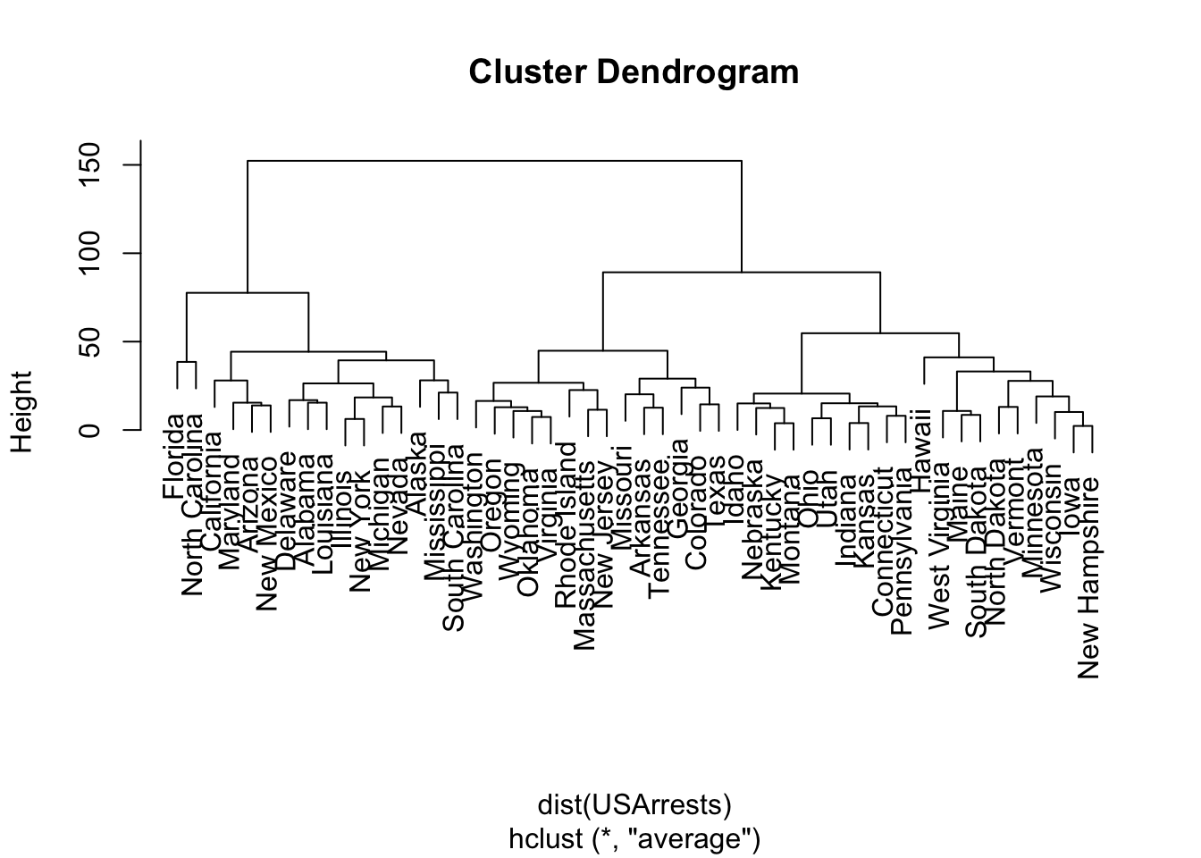
##
## hclust> plot(hc, hang = -1)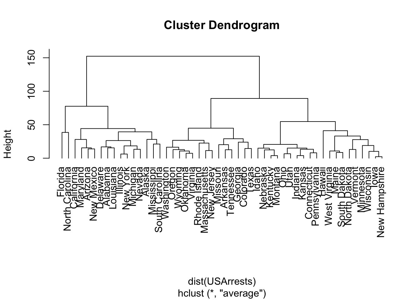
##
## hclust> ## Do the same with centroid clustering and *squared* Euclidean distance,
## hclust> ## cut the tree into ten clusters and reconstruct the upper part of the
## hclust> ## tree from the cluster centers.
## hclust> hc <- hclust(dist(USArrests)^2, "cen")
##
## hclust> memb <- cutree(hc, k = 10)
##
## hclust> cent <- NULL
##
## hclust> for(k in 1:10){
## hclust+   cent <- rbind(cent, colMeans(USArrests[memb == k, , drop = FALSE]))
## hclust+ }
##
## hclust> hc1 <- hclust(dist(cent)^2, method = "cen", members = table(memb))
##
## hclust> opar <- par(mfrow = c(1, 2))
##
## hclust> plot(hc,  labels = FALSE, hang = -1, main = "Original Tree")
##
## hclust> plot(hc1, labels = FALSE, hang = -1, main = "Re-start from 10 clusters")
##
## hclust> par(opar)
##
## hclust> ### Example 2: Straight-line distances among 10 US cities
## hclust> ##  Compare the results of algorithms "ward.D" and "ward.D2"
## hclust>
## hclust> mds2 <- -cmdscale(UScitiesD)
##
## hclust> plot(mds2, type="n", axes=FALSE, ann=FALSE)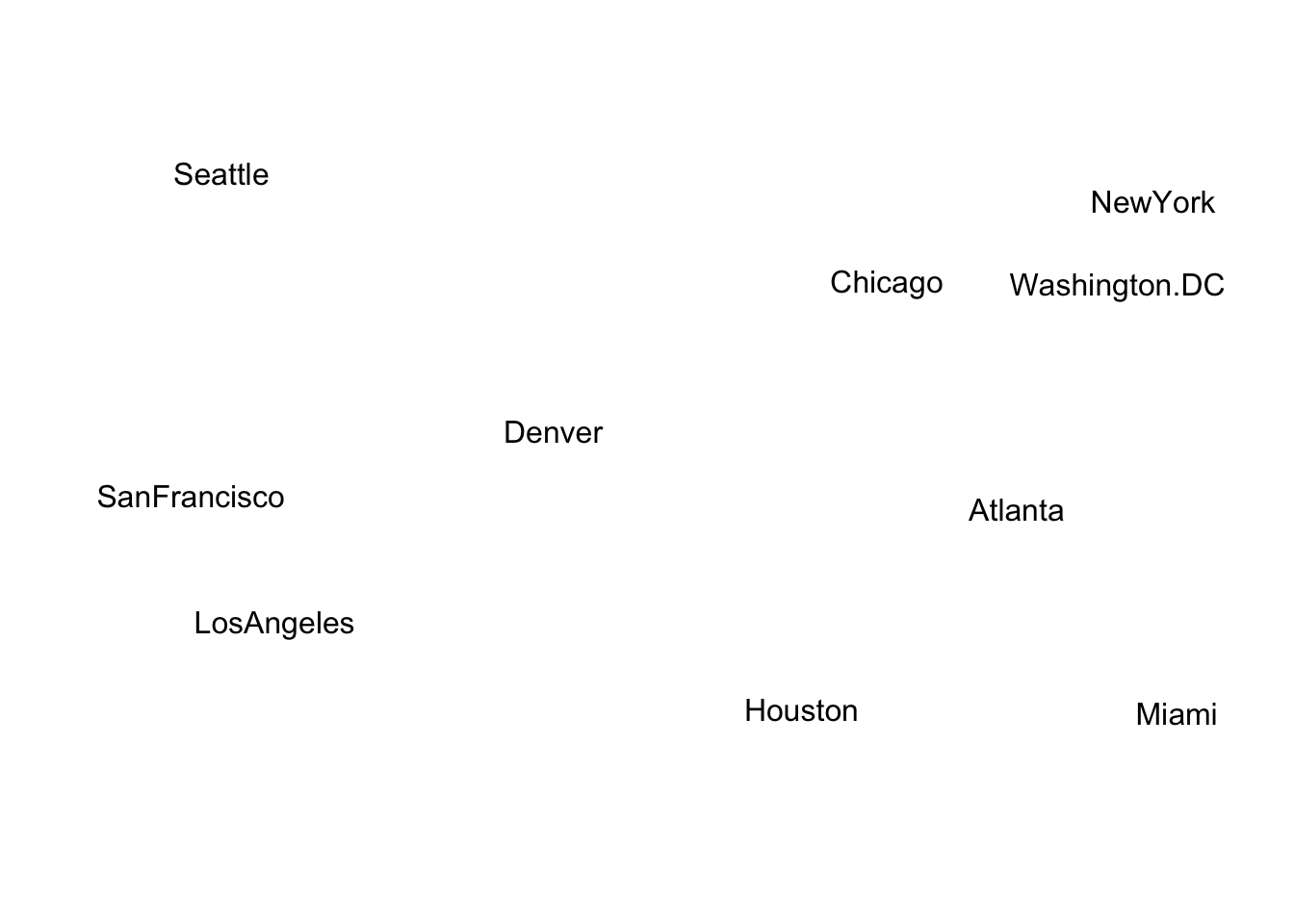
##
## hclust> text(mds2, labels=rownames(mds2), xpd = NA)
##
## hclust> hcity.D  <- hclust(UScitiesD, "ward.D") # "wrong"
##
## hclust> hcity.D2 <- hclust(UScitiesD, "ward.D2")
##
## hclust> opar <- par(mfrow = c(1, 2))
##
## hclust> plot(hcity.D,  hang=-1)
##
## hclust> plot(hcity.D2, hang=-1)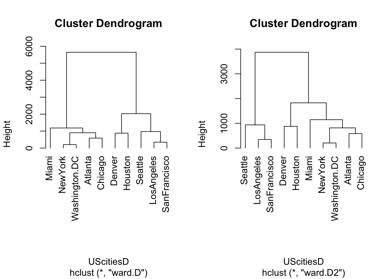
##
## hclust> par(opar)
Todo lo anterior requiere que conzocamos el nombre correcto del comando, pero ¿qué pasa si no lo sabemos?
Podemos utilizar el comando apropos() para encontrar todo lo relacionado con algún término
apropos("solve")## [1] "backsolve" "forwardsolve" "qr.solve" "solve"
## [5] "solve.default" "solve.qr"
2.3 Expresiones y asignaciones
Hay dos tipos de resultados en R: expresiones y asignaciones. Las primeras sólo se muestran a la salida estándar y NO se guardan en una variable; las segundas, se asignan y guardan en una variable
Expresión:
rnorm(10)## [1] 0.7979605 1.0878395 -0.6359152 0.4398236 0.8196364 0.1650391
## [7] -0.5915663 0.7436936 -0.1450920 -1.1731611Asignación
x <- rnorm(10)
x## [1] 0.99989450 2.42087085 -0.51606105 -0.97184273 1.37932604 -0.72765265
## [7] -1.08607929 0.03003202 -0.87025071 -2.27234173
Operado de asignación. Evitar el uso del igual
R distingue entre mayúsculas y minúsculas, así las siguientes variables contienen valores distintos
a <- 3
A <- 6Los comandos pueden separarse por ; o - mejor opción- por un salto de línea
a <- 3; b <-5también pueden definirse asignaciones en más de una línea
a <-
  pi + 12
2.4 Movimiento entre directorios
Para saber en qué directorio estamos tecleamos
getwd()## [1] "/Users/robertoalvarez/Dropbox/UAQ/Bioinformatica/Introduccion-a-R.github.io"Para cambiar de directorio utilizamos setwd("direccion_a_la_que_quieres_ir")
setwd("~")También podemos usar los comandos de bash dentro de R, utilizando la función system()
system("ls -la")
system("pwd")2.5 Importante
Como regla general todos los nombres van entre comillas: nombre de carpetas, archivos, de columnas, de renglones,etc.
2.6 Operaciones aritméticas
Se puede sumar, restar, multiplicar,dividir, “exponenciar” y calcular la raíz cuadrada.
Los operadores son, respectivamente: +,-,*, /,** o ^, sqrt()
a + b## [1] 20.14159
a - b## [1] 10.14159
a * b## [1] 75.70796
a ** b## [1] 795898.7
a ^ b## [1] 795898.7
sqrt(a)## [1] 3.891222.7 Prioridad en las operaciones
Las operaciones se efectuan en el siguiente orden:
- izquierda a derecha
- sqrt() y ** , ^
- “*” y /
- “+” y -
- <-
Este orden se altera si se presenta un paréntesis. En ese caso la operación dentro del paréntesis es la que se realiza primero.
Ejemplos
4 + 2 *3 = 4 + 6 = 10
4-15/3 +3^2 +sqrt(9)= 4-15/3 + 9 +3 = 4-5+12=13
4-(3+7)^2 + (2+3)/5=4-100+5/5=-95
2.8 Tipos de datos lógicos o booleanos
Estos tipos de datos sólo contienen información TRUE o FALSE. Sirven para evaluar expresiones de =, <, > y pueden utilizarse para obtener los elementos de un vector que cumplan con la característica deseada.
1 < 5## [1] TRUE
10 == 0 # Es igual a## [1] FALSE
10 != 0 # NO es igual a## [1] TRUE
10 <= 0 #Menor o igual ## [1] FALSEDentro de R un valor lógico TRUE equivale a 1 y FALSE equivale a 0, por lo tanto para contar cuántos TRUEs hay podemos hacer una suma:
Ejercicio utiliza una sola líndea de R para averiguar si el logaritmo base de 10 de 20 es menor que la raiz cuadrada de 4.
2.8.1 Caracter
Son strings de texto. Se distingue porque los elementos van entre comillas (cada uno). Puede ser desde un sólo caracter hasta oraciones completas. Puede parecer que contienen números, pero las comillaa indican que serán tratados como texto. Podemos subsetearlos por su índice o buscando literalmente el texto.
x<- "La candente mañana de febrero en que Beatriz Viterbo murió, después de una imperiosa agonía que no se rebajó un solo instante ni al sentimentalismo ni al miedo"2.8.2 Enteros y números (numeric)
R por default representa los números como numeric, NO integer. Estos tipos son dos formas diferentes en las cuales las computadoras pueden guardar los números y hacer operaciones matemáticas con ellos. Por lo común esto no importa, pero puede ser relevante para algunas funciones de Bioconductor, por ejemplo ya que el tamaño máximo de un integer en R es ligeramente más chico que el tamaño del genoma humano.
¿Cómo revisar si un objeto es numeric o entero?
x <- 1
class(x)
## [1] "numeric"
x <- 1:3
class(x)
## [1] "integer"